As global data creation continues to accelerate toward a projected 175 zettabytes by 2025, the demand for high-performance data processing frameworks has never been more critical. Apache Spark, and specifically its Python API, PySpark, has emerged as the industry standard for managing massive datasets across distributed clusters. However, the transition from small-scale experimentation to enterprise-level production often reveals significant performance bottlenecks. Without rigorous optimization, Spark jobs frequently suffer from excessive shuffling, memory overflows, and inefficient resource utilization, leading to inflated cloud infrastructure costs and delayed business insights.

To address these challenges, data engineers utilize a suite of sophisticated techniques designed to harmonize code execution with Spark’s underlying architectural mechanics. Understanding how Spark executes code is the prerequisite for any optimization effort. Spark operates on a master-slave architecture where a Driver program coordinates tasks executed by multiple Workers (Executors). By leveraging a Directed Acyclic Graph (DAG) and the Catalyst Optimizer, Spark attempts to streamline execution plans. However, the human element—the way the code is written—remains the primary determinant of system efficiency.
The Foundation: Understanding Execution Mechanics
The core of Spark’s efficiency lies in two concepts: Lazy Evaluation and the abstraction of Transformations and Actions. Transformations, such as filter() or select(), do not trigger immediate computation. Instead, Spark records these operations as a logical plan. Only when an Action, such as count(), show(), or write(), is invoked does the Spark engine compile the logical plan into a physical plan for execution.
This “lazy” approach allows the Catalyst Optimizer to perform “predicate pushdown” and “column pruning,” effectively removing unnecessary data before it ever reaches the memory of an executor. For developers, the first step in optimization is often using the .explain() method. This tool provides a transparent view of the execution plan, highlighting whether filters are being applied at the source level or if the system is performing expensive shuffles.
1. Transitioning to Columnar File Formats
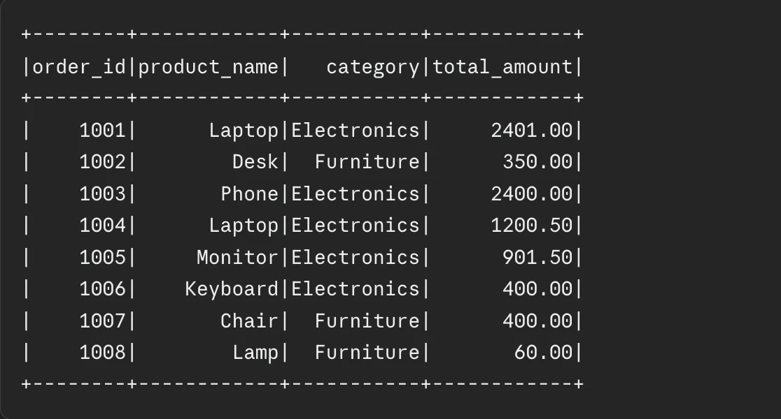
The choice of file format is perhaps the most impactful decision in the data ingestion phase. While CSV and JSON are human-readable and widely used for small datasets, they are row-based formats that force Spark to read every column in a row even if only one is required. This results in significant I/O overhead.
In contrast, columnar formats like Apache Parquet and ORC (Optimized Row Columnar) store data by columns. This allows Spark to skip irrelevant data entirely. Furthermore, Parquet files store metadata, including minimum and maximum values for each column within a row group. This enables “dictionary encoding” and “bit packing,” which drastically reduce the storage footprint and increase read speeds. Industry benchmarks consistently show that switching from CSV to Parquet can reduce storage requirements by up to 75% while improving query performance by a factor of ten.
2. Implementing Predicate Pushdown and Early Filtering
The principle of “filtering early” is fundamental to distributed computing. By applying filters immediately after loading a dataset, engineers reduce the volume of data that must be moved across the network or stored in memory. Predicate pushdown takes this a step further by moving the filter logic directly into the file-reading metadata.
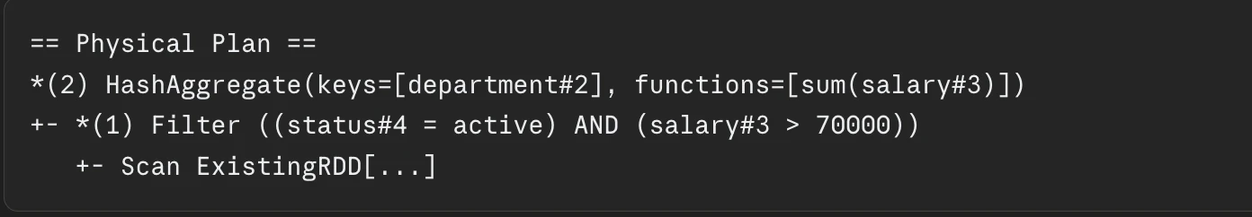
For instance, if a query seeks sales data only for the year 2023 from a Parquet source, Spark can use the file metadata to ignore all data blocks that do not contain the “2023” value. This minimizes the “Shuffle” phase—the most expensive part of any Spark job—by ensuring that only relevant records participate in downstream joins or aggregations.
3. The Power of Column Pruning
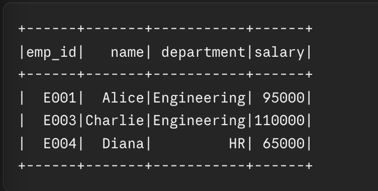
In many enterprise environments, DataFrames can contain hundreds of columns. If a data pipeline only requires five of those columns for a specific calculation, reading the remaining 95 is a waste of CPU and memory. Column pruning is the process of explicitly selecting only the necessary fields using the .select() statement. When combined with columnar formats, Spark avoids loading the discarded columns into memory altogether, further reducing the pressure on the Java Virtual Machine (JVM) heap.
4. Optimizing Partition Strategy
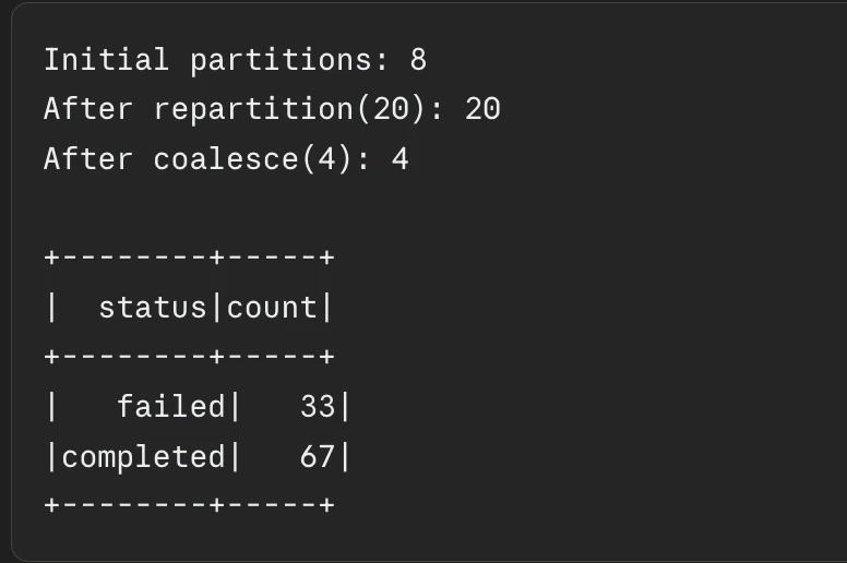
Partitioning determines how data is distributed across the cluster. If partitions are too large, a single executor may run out of memory (OOM error). If they are too small, the overhead of managing thousands of tiny tasks can overwhelm the Driver.
The general consensus among data engineers is to aim for 128MB to 200MB per partition. Spark provides two primary methods for adjusting this: repartition() and coalesce(). While repartition() performs a full shuffle to increase or decrease the number of partitions, coalesce() is a more efficient way to reduce the number of partitions because it minimizes data movement across the network.
5. Leveraging Broadcast Joins for Small Tables
Joins are notoriously resource-intensive because they typically require a “Sort Merge Join,” which involves shuffling both datasets across the network so that matching keys end up on the same executor. However, if one of the tables is small enough to fit into the memory of each executor (typically under 10MB by default, though this can be tuned), a Broadcast Join can be used.
In a Broadcast Join, Spark sends a full copy of the small table to every executor. This allows the join to happen locally on each machine, eliminating the need for a shuffle. This technique can reduce the execution time of a join from minutes to seconds.
6. Enabling Adaptive Query Execution (AQE)
Introduced in Spark 3.0, Adaptive Query Execution is a dynamic optimization layer that re-optimizes the execution plan based on runtime statistics. Before AQE, Spark’s execution plan was static. With AQE enabled, Spark can:
- Coalesce shuffle partitions: Automatically merge small partitions after a shuffle to avoid task overhead.
- Switch join strategies: Change a Sort Merge Join to a Broadcast Join if it realizes at runtime that one side of the join is small enough.
- Optimize skew joins: Detect if data is unevenly distributed and break down large partitions to balance the load.
7. Avoiding Python UDFs in Favor of Native Functions
One of the most common pitfalls in PySpark is the over-reliance on Python User Defined Functions (UDFs). Because Spark’s core is written in Scala and runs on the JVM, executing a Python UDF requires Spark to serialize data, send it to a Python process, execute the function, and then send the result back to the JVM. This “SerDe” (Serialization-Deserialization) overhead is massive.

Data engineers are encouraged to use pyspark.sql.functions, which are optimized, compiled expressions that run directly within the JVM. For complex logic that cannot be handled by native functions, “Pandas UDFs” (Vectorized UDFs) provide a more efficient alternative by using Apache Arrow to transfer data in batches rather than row-by-row.
8. Strategic Data Caching and Persistence
Caching is a double-edged sword. While .cache() or .persist() can store a DataFrame in memory for reuse, over-caching can lead to memory pressure and “spilling” to disk, which is significantly slower. The rule of thumb is to cache a DataFrame only if it is accessed multiple times in the pipeline (e.g., in a loop or by multiple downstream branches). It is equally important to use .unpersist() once the data is no longer needed to free up cluster resources.
9. Managing Data Skew through Salting
Data skew occurs when a few keys in a dataset have significantly more records than others (e.g., a “Null” key or a very popular product ID). This causes a few executors to work much harder and longer than others, creating a bottleneck. “Salting” is a technique where a random integer (the “salt”) is added to the join key to break up large partitions. After the join or aggregation is performed, the salt is removed to restore the original key structure. This ensures a more uniform distribution of work across the cluster.
10. Minimizing Shuffle Operations
Shuffling is the “silent killer” of Spark performance. It involves disk I/O, data serialization, and network transfer. Engineers should aim to reduce the number of shuffles by combining multiple transformations into a single stage. For example, instead of performing multiple groupBy operations on different columns sequentially, it is often more efficient to perform a single groupBy on multiple columns or use window functions to achieve the same result with less data movement.

11. Implementing Bucketing for Repeated Joins
For large datasets that are joined frequently on the same key, “Bucketing” offers a long-term solution. By pre-sorting and partitioning data on disk based on a specific column, Spark can perform joins without any shuffling. When two bucketed tables are joined on their bucketed column, Spark simply matches the corresponding files. This is particularly effective in data warehousing environments where large “fact” tables are joined daily with “dimension” tables.
12. Fine-Tuning Spark Configurations
The final layer of optimization involves tuning the Spark environment itself. Key configurations include:
spark.executor.memory: Allocating enough memory to avoid disk spilling.spark.memory.fraction: Controlling the balance between execution memory and storage memory.spark.sql.shuffle.partitions: Adjusting the default (200) to match the actual size of the data and the number of available CPU cores.spark.serializer: UsingKryoSerializer, which is more compact and faster than the default Java serializer.
Chronology of Spark Performance Evolution
The journey toward these optimization techniques has been marked by several milestones in the Apache Spark project. In 2014, Spark 1.0 introduced the basic RDD (Resilient Distributed Dataset) API. However, the release of Spark 2.0 in 2016 was a turning point, introducing the DataFrame API and the second-generation Tungsten execution engine, which optimized memory management and code generation.
The most significant leap for PySpark users came with Spark 3.0 in 2020, which brought Adaptive Query Execution and improved Pandas UDFs. Subsequent updates, including Spark 3.2 and 3.5, have focused on “Connect” architectures and further enhancing the integration between Python’s data science ecosystem and Spark’s distributed power.
Implications for the Industry
The implications of these optimizations extend beyond mere technical efficiency. For organizations operating at the petabyte scale, a 20% improvement in Spark job efficiency can translate into millions of dollars in annual cloud savings. Furthermore, as sustainability becomes a corporate priority, reducing the computational intensity of data pipelines directly lowers the carbon footprint of data centers.
Experts in the field suggest that as Spark continues to evolve, the boundary between “writing code” and “tuning infrastructure” will continue to blur. The rise of “Serverless Spark” offerings from major cloud providers (AWS Glue, Google Cloud Dataproc Serverless, and Azure Synapse) automates some of these optimizations, yet a deep understanding of partitioning, shuffles, and memory management remains the hallmark of a senior data engineer.
In conclusion, PySpark optimization is an iterative process of monitoring, analyzing, and refining. By implementing these 12 techniques—ranging from choosing the right file format to mastering the nuances of data skew—engineers can transform sluggish, expensive data jobs into streamlined, high-performance pipelines capable of meeting the demands of the modern data era.